A Low-Pass Filter Guide for Non-DSP Engineer
A simple implementation of C++ digital Low-pass filter
Life without powerful DSP tools like MATLAB can be very tough, especially for those engineers who need to process real-world data in the production env. Digital filtering on continuous data is a very common use case in a lot of User Interface rendering. Among all the digital signal processing techniques, the low-pass filter is the most fundamental one and can smooth out noise or unwanted jittering in the data sequence. This article will discuss designing a C++ Low-pass filter from scratch.
- Digital Filter Basics
- Low-pass Filter
- S-Domain
- Z-Domain
- Digital Representation of the Filter
- C++ code for 3rd-order Butterworth Filter for a float sequence
- Phase Compensation
- Other Curve Smoother algorithms
Digital Filter Basics
Filter designing is all about needs. There are so many choices and parameters to tweak. Knowing the design requirements is very important before we even start. Some typical digital filter spec parameters are passband cutoff frequency, stopband cutoff frequency, peak ripple, attenuation, and gain. The definition of the cutoff frequency is the frequency which gain magnitude drop by -3dB.
There are basically 2 types of digital filters: Infinite-Impulse Response filter and Finite-Impulse Response filter.
| IIR | FIR |
| Designed base on the feedback loop, not guaranteed to be stable | Designed base on a sliding window. Hard to design but stable. Image Gaussian Blur can be understand as a 2D FIR filter |
| IIR is usually faster in response because the feedback loop design | FIR usually worse than the IIR under the same order |
| IIR design you can read the rest of this article | FIR kernel design you can use the scipy python package |
Also, we cannot break the law of Physics. So there must be some delay in the digital filtering in the time domain. The delay is correlated with the order of the filter. For example, if the order is 3, then we are expected to see 3 frames of delay. To obtain the full sequence of the processed data, we need to have some phase compensation for the delay at the end. Also the higher the order, the faster the response damping.
Reads:
Low-pass Filter
Low-pass filter is a filter that only allows low-frequency components in the signal to pass. We can use it to remove spikes in the curve, erase high-frequency component to blur images, and denoising in the audio. Other formats of filters like High-pass or Band-pass are designed in a similar fashion. So we only focus on the Low-pass Filter in this article.
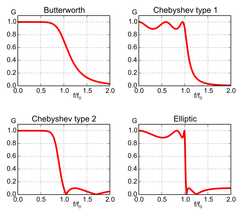
There are multiple formats of Low-pass Filter. The most common 2 types are Butterworth and Chebyshev. The difference between them is that they have different mathematic formulas to characterize the frequency response curve.
| Butterworth | Chebyshev Type I |
 |  |
| Slow damping | Faster damping, but has ripple |
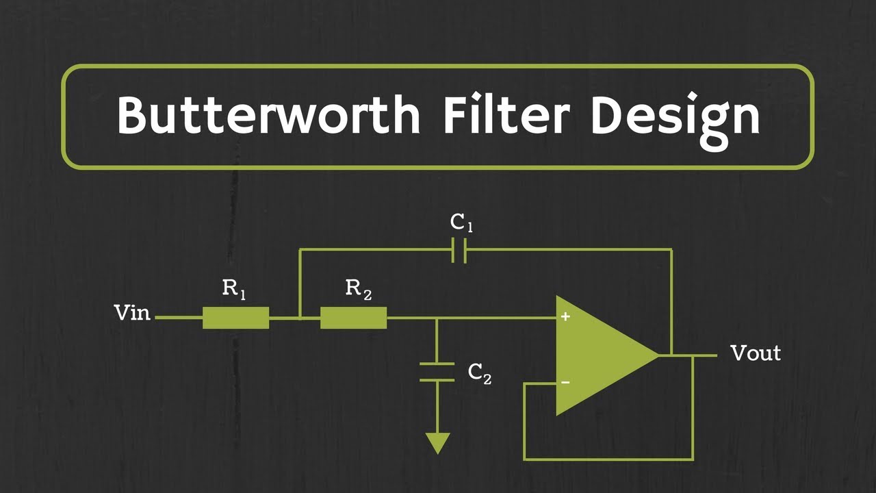
Here we choose Butterworth Low-pass filter. To design a Butterworth we just need the number of the order N and the Cutoff frequency Wc. Or we can use the passband cutoff and stopband cutoff to calculate the N and Wc.
Notice that when the Butterworth order is 2, the filter is also called Biquad filter. It is very handy to cascade and builds filter blocks.
The Bode plot of the Butterworth Low-pass filter and others can be found below. From the above frequency response formula, we can see that when w = Wc, the gain is 0.707 which is -3dB. Also the higher the frequency, the lower the gain.
Reads:
- Low-pass filter - Wikipedia
- Butterworth filter - Wikipedia
- Chebyshev filter - Wikipedia
- Digital biquad filter - Wikipedia
S-Domain
In the above section, we design our Butterworth filter in the frequency domain, this is because it is straightforward to characterize the response curve function to meet our requirement in the frequency domain. However, when implementing the actual digital filter in the LTI system, engineers usually analyze the transform function in the S-domain. We can perform Nyquist stability criterion analysis in the S-domain. Also as our data is digital which is discrete, so we will also perform the Z-transform to convert the transfer function to the Z-domain.
To determine the transfer function in the S-domain, we need to use the frequency domain’s property: Complex Conjugate Symmetric. We then obtain this constraint equation:

Then we solve the equation to find out the poles for the transfer function H(s) and H(-s). To keep the system stable, we only select the poles in the negative real half-plane of S-domain. Then eventually we can write down the transfer function in the S-domain based on:

Probably you like me, already lost in the last paragraph. A good thing is there is a normalized format of this transfer function base on the order of the filter. You can find the reference chart here: Butterworth filter - Wikipedia. To use this we just need to select an order and substitute the s with s/Wc. Now we successfully have our Low-pass filter in the S-domain as H(s).
Reads:
- Butterworth filter - Wikipedia
- Laplace transform - Wikipedia
- s-plane - Wikipedia
- Nyquist stability criterion - Wikipedia
Z-Domain
Since the H(s) we obtained are analog filters, we need to map it to the discrete Z-Domain to obtain a digital filter. The common methods are the Impulse Invariance and the Bilinear Transform. Here we using Bilinear Transform, which is the first-order Taylor Series approximation to map S-domain to Z-domain. Once we are in the Z-domain, it is very easy to convert the filter to a digital circuit or the software algorithm.
Bilinear Transform is just substituting the s in the H(s) to this:

The Z-domain representation of a Biquad Low-pass filter is:
A complete example can be found in the EarLevel article
Reads:
Digital Representation of the Filter
Now we need to do is converting this discrete domain filter into a logic block network. There are multiple design principles here, like the Direct form and the Transposed Direct form. Either form of design can work, the major difference is how much actual logic blocks the form will use. The Z^-1 is the delay block. In order to reduce the number of delay blocks, we can use the Transposed Direct-Forms II design. So we can reduce the memory usage of the filter. The logic block diagram is:
![]()
Using the above diagram, we can convert the Z-domain system Transfer function into a difference equation. The following is the Biquad Difference Equation.

We can resolve the unknown parameters a and b. Then replace it inside the difference equation, then we have our final digital Low-pass filter in the time domain.
Reads:
C++ code for 3rd-order Butterworth Filter for a float sequence
constexpr float Wc = 0.2f; // cutoff frequency in rad/s
constexpr float K = std::tan(M_PI * Wc);
float norm = 1 / (K*K*K + 2*K*K + 2*K + 1);
float a0 = K*K*K*norm;
float a1 = 3 * a0;
float a2 = a1;
float a3 = a0;
float b1 = (3*K*K*K + 2*K*K - 2*K - 3) * norm;
float b2 = (3*K*K*K - 2*K*K - 2*K + 3) * norm;
float b3 = (K*K*K - 2*K*K + 2*K - 1) * norm;

// z and p are the delay memory blocks
bool onReceiveData(float input, float& output) {
  float output = input * a0 + z1;
  z1 = input * a1 + z2 - b1 * output;
  z2 = input * a2 + z3 - b2 * output;
  z3 = input * a3 - b3 * output;
  p0 = p1; p1 = p2; p2 = input;

  // Since LPF is not stable on first N frame
  // 1) we need to bypass input at first N-3 frames
  // 2) cache input between [N-3, N), no output at all
  // 3) between [N, N+3), we need to blend the output with the cached inputs with index based weights
  // 4) for following frames, we can use the LPF normally
}

std::vector<float> getPhaseCompensation() {
  // return latest 3 inputs, since they are not processed
  return {p0, p1, p2};
}
Reads:
Phase Compensation
Since we are using the 3rd Order filter, we will have a delay of 3 frames. So when finishing input data, the output stream is still lagging by 3 frames. We need to manually pull the data from the queue.
Also, IIR filter might not work well at the beginning. For the first several frames, we need to use the original input data. Also when it starts taking effect, we should blend the first 3 filter output with the cached original input to avoid phase shifting.
Now we can use our little filter smooth out any high frequency noise data.
Other Curve Smoother algorithms
We can also downsampling the original data and smooth it through the spline approximate functions group. Or we can even select some key points and using the segmented Bezier Curve to approximate a smooth curve. Other types of filter like Kalman Filter can also smooth the curve. We will discuss Kalman Filter in the up coming blog.