SLAM Knowledge Tree
in 3D Vision
Knowledge Tree for SLAM
This post records knowledge structure for the 3D Computer Vision. This post will emphasis on the SLAM technology, which is machine perception and mapping in unknown environment. There is another post that emphasis on Structure from Motion, which talks more about some fundamental concepts SfM Knowledge Tree.
- SLAM Overview
- SLAM Comparison with SfM
- Feature based Visual Odometry
- Optical Flow Visual Odometry
- Sensor Fusion
- Backend Optimization
- Loop Closure
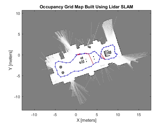
- Mapping
- Misc
- Overview
- Resources
- CV Basics
- Deep Learning
- Deep Learning in Computer Vision
- Graph Representation Learning
- Sensor Fusion
- Pose Estimation Model
- Mapping
- Non-linear Optimization
- SLAM framework in depth
- Deep Learning SLAM
Updated on Mar 28, 2021
SLAM Overview
- Visual Odometry
- Sensor Fusion
- Backend Optimization
- Loop Closure
- Mapping
A overall SLAM system design can be see in this ORB-SLAM2 diagram: 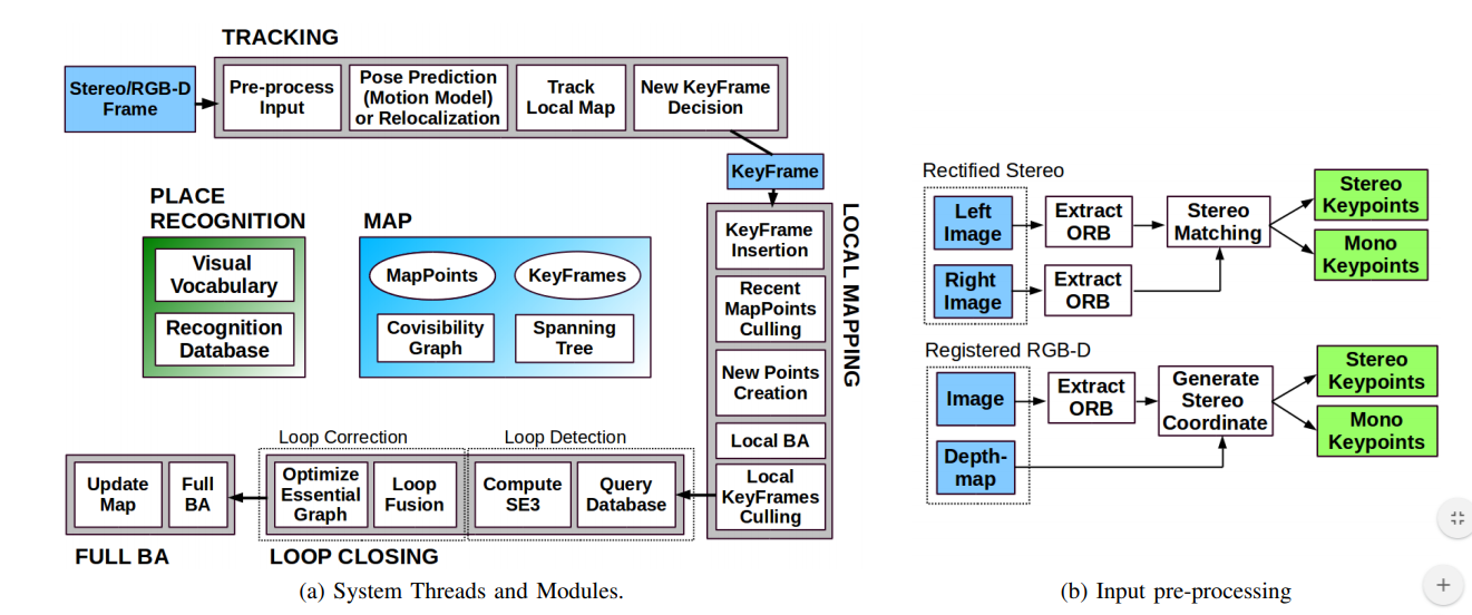
SLAM Comparison with SfM
- SLAM require to be real-time while SfM can be offline.
- SfM also doesn’t require the image data to be in time sequence, while in SLAM data always arrive in sequence.
- SfM can apply RANSAC across the whole image data set to perform triangulation, while SLAM can match the features between current frame and previous reference frame or built map.
- SfM is batch operation while SLAM is incremental.
- SfM can perform non-linear optimization across the whole Bundle Adjustment graph, while SLAM usually only update the partial graph.
- SfM 3D Reconstruction require accurate mesh reconstruction and texture mapping, while SLAM map can be point cloud or other simplified format.
Feature based Visual Odometry
- VO is vision based method which the observed data is the camera data and use it to estimate the hidden camera pose and motion state. Also usually assume the intrinsic matrix is known.
- Feature Detection:
- ORB
- FAST + BRIEF
- Subpixel refinement
- Feature refinement, when paired features are not on the same Epiplane:
- Minimize Sampson Distance
- Mid-point Triangulation
- ORB
- The solution of recovering the [R, t] is various based on the type of the camera sensor:
- Monocular initialization (Need camera pose has translation)
- 2D-2D: Epipolar constraint, Linear algebra solution, 8-points algorithm
- Essential Matrix
- Homogeneous Matrix
- 2D-2D: Epipolar constraint, Linear algebra solution, 8-points algorithm
- Stereo and RGB-D, or image with map
- 2D-3D: PnP
- Direct Linear Method with SVD, n = 6
- P3P, Linear method, n = 3
- EPnP, linear Method, n = 4
- Non-Linear: Bundle Adjustment, minimize reproduction error.
- Construct the least square reprojection error function.
- Calculate the Analytic Partial Derivative for both pose and landmark (Jacobian)
- Use the above linear method output as the initial BA state.
- Optimize both Pose and Landmark using the non-linear optimization algorithm like LM
- Each edge will update the vertices connect to it for certain amount of epoch until converge.
- 3D-3D point cloud: ICP
- Linear method: SVD
- Non-Linear: BA
- 2D-3D: PnP
- Lidar
- Nearest Neighbor
- Monocular initialization (Need camera pose has translation)
- Keyframe
- When initialization, the # of detected feature points need to larger than a threshold to be consider as initialization success
- During SLAM, the definition of a keyframe is: the delta of pose [R, t] with the last keyframe is larger than a threshold
Optical Flow Visual Odometry
- Optical Flow can avoid feature detection and feature matching. Basic idea is to assume the camera transform across frame is really small. So that we can have the strong assumption: Grayscale invariant. So that each pixel can be considered as a feature point.
- Linear Solution: LK Optical Flow, still need to detect feature at first frame and does the feature tracking. Still rely on PnP etc to recover the pose
- Non-linear Solution: Direct Method, which also is BA. Can optimize the pose and the landmark map. Map can be Sparse, Semi-dense, or Dense. This is also used for Dense Reconstruction.
Sensor Fusion
- Use other sensor’s data to constraint the camera motion. E.g. use IMU data for the state update, so that we can better predict the camera pose in the map for PnP
Backend Optimization
- Backend can refine the front-end rough estimation. It works by define a parametric least square Loss function. And update the state variables to find argmin(state) of the global minimum of the Loss function. The main part of this optimization flow is to find the direction of the gradient to each state variable (Jacobian Matrix) at the current state. Then update the state along that Gradient Descent direction.
- Filter-based method: Extened Kalman Filter
- Will post another blog for KF
- Bundle Adjustment: Non-linear Optimization
- First order Gradient Descent.
- Second order Gradient Descent (Newton method)
- Approximation to the Second Order Gradient Descent
- Gaussian-Newton method
- Levenberg-Marquardt: Trust region based gradient descent.
- Filter-based method: Extened Kalman Filter
Loop Closure
- Bag-of-words
- Deep Learning based.
Mapping
- Only insert the feature points on the keyframe to the map
- Every time detect a loop closure, optimize the whole BA graph
Misc
- Left/right Perturbation
- Taylor Series
- Regulation term in loss function: convert the constraint based problem to no constraint problem.
- Marginalization: Schur Complement.
Overview
- General categories
- System: Monocular, Stereo, RGB-D, VIO, LiDAR.
- VO: 2D-2D, 2D-3D, 3D-3D
- LiDAR: scan-scan, scan-map
- IMU & GPS: Pre-integration, Difference method
- Reconstruction: Sparse, Semi-dense, Dense
- Other topics: Object detection, Semantic Segmentation, etc.
- Milestone works
- PTAM 2007
- DTAM 2011
- ORB-SLAM2 2017
- VINS-Mono 2017
- DSO 2016
- PL-VIO 2018
- DL driven:
- DVSO 2018
- CNN-SLAM 2018
- Multi-Geometry Features
- Feature Points
- Versatile to lighting
- May lose tracking
- Feature Line
- Feature Plane
- Deep Learning Features
- Feature Points
Resources
- Frameworks/Libraries
- OS: ROS
- Math: Eigen
- CV: OpenCV, PCL
- Optimization: g2o, Ceres, gtsam, PyTorch Geometric
- Graphic: OpenGL, Pangolin
- Features: libpointmatcher, DBow2
- Mapping: OctoMap, OpenFABMAP
- Open-source projects
- GitHub - yanyan-li/SLAM-BOOK
- GitHub - wuxiaolang/Visual_SLAM_Related_Research
- GitHub - raulmur/ORB_SLAM2: Real-Time SLAM for Monocular, Stereo and RGB-D Cameras, with Loop Detection and Relocalization Capabilities
- GitHub - UZ-SLAMLab/ORB_SLAM3: ORB-SLAM3: An Accurate Open-Source Library for Visual, Visual-Inertial and Multi-Map SLAM
- GitHub - colmap/colmap: COLMAP - Structure-from-Motion and Multi-View Stereo
- GitHub - JakobEngel/dso: Direct Sparse Odometry
- GitHub - RobustFieldAutonomyLab/LeGO-LOAM: LeGO-LOAM: Lightweight and Ground-Optimized Lidar Odometry and Mapping on Variable Terrain
- GitHub - mapillary/OpenSfM: Open source Structure-from-Motion pipeline
- GitHub - tum-vision/lsd_slam: LSD-SLAM
- GitHub - HKUST-Aerial-Robotics/VINS-Mono: A Robust and Versatile Monocular Visual-Inertial State Estimator
CV Basics
- Feature Fitting
- RANSAC: Random Sample Consensus
- J-Linkage
- T-Linkage
- Feature Points: SIFT, ASIFT, SURF, ORB
- SIFT:
- DoG(Difference of Gaussians) to get image information at different frequency level, aka Gaussian Pyramid.
- Find initial feature points in 3-dimensional Gaussian Pyramid, which are the local maximum or minimum of the 26 surrounding points.
- Remove outlier feature points at the edge. Also refine the feature points position
- Calculate the Gradient Direction of the feature point based on the 4 directional pixels around it at the same Gaussian Pyramid level.
- Build Descriptor: select the kernel of 16x16 around the key point. For every 4x4 sub-kernel, build the gradient histogram. Each bin represent gradient direction within 45 degree (8 bins). There are 16 sub-kernel. So we have a 128-dim vector descriptor
- For larger rotation between 2 frames, we can use ASIFT
- SURF:
- Main difference with SIFT is the descriptor
- ORB:
- FAST corner point
- For all points. Select the 16 points at the circle of radius 3 around the point.
- It is a feature point if there are more than N (usually 12) points on that circle is larger or smaller than the point’s color with a threshold.
- Pass the feature point to a decision tree to trim bad features
- After iterate across the image, select feature points of top-N Harris Response.
- ORB also take care of the Scale-invariant by using Gaussian Pyramid and detect FAST at each level
- For Rotation-invariant, ORB use Intensity Centroid. The gradient direction is defined as the direction from feature point to the centroid of a small kernel around it.
- BRIEF descriptor
- Select a kernel around the feature point. Random select point pairs within the kernel. Use binary to represent the comparison between the 2 points. So we have a binary 128-dim vector descriptor
- Pair Selection can base on 2D Gaussian distribution
- Steer BRIEF: apply rotation to the pair selection mask base on the Intensity Centroid calculated in FAST
- FAST corner point
- Feature Points Matching across 2 frames
- Brute-force
- Hamming Distance
- FLANN
- SIFT:
- Feature Line
- Hough Transform
- LSD: cv::line_descriptor. Note this is not LSD-SLAM
- Feature Plane
- Extracting plane from Point Cloud
- Calculate normal for each 3D point, based on the surrounding 3D points and prior info
- Clustering points with similar normal direction
- AHC: Agglomerative Hierarchical Clustering. A better open-source solution
- Plane Matching based on normal + distance between origin and the plane
- Extracting plane from Point Cloud
- Feature Constraints
- Vanishing Point Constraint: parallel lines on the image will be merged at a point, due the perspective projection
- Vanishing Point is used for online calibration
- Vanishing Line Constraint: a 3D space plane’s intersection line with the camera plane. Any set of lines parallel to the 3D space plane, their vanish point will be on the vanishing line.
- Manhattan World Constraint: Our world usually is build with 3 perpendicular planes
- Same Plane Constraint: for feature point/line on the same plane, they will maintain the constraint across frames
- Vanishing Point Constraint: parallel lines on the image will be merged at a point, due the perspective projection
Deep Learning
- Popular Architectures: VGG, ResNet, DenseNet, AlexNet, GoogleNet, MobileNet, U-Net
- Network design Tips:
- 1x1 convolution kernel: use to adjust the tensor size. Whether reduce or increase depend on the number of the filters
- Residual module can solve the issue of gradient explosion/diminish
- After ReLU, need to add a local response normalization layer to rectify the tensor data. This is normalize the output (feature map) of all neurons in 1 layers for 1 sample
- Batch Normalization: normalize the output of same neuron across all the samples in 1 mini batch.
- Gradient Descent Optimizer
- SGD + Momentum
- Adaptive Learning rate: Adam, RMSProp, AdaDelta
- Model Evaluation:
- Precision and Recall: ROC, AUC
- Accuracy
Deep Learning in Computer Vision
- Feature Point Prediction: GCNv2
- Feature Line Prediction
- Object Detection
- Bounding Box
- Instance Segmentation
- Obtain depth map from monocular frame
- FCN: Fully Convolutional Networks for Semantic Segmentation
- Deconvolution: Padding original tensor to bigger size and do a normal convolution, such that output is larger than original tensor size
- CRF: conditional random field
- CNN-SLAM: not real-time
- MobileNet V2: decompose convolution to depth-wise convolution and 1x1 convolution
- GeoNet: consider normal map and depth map together
- Unsupervised Learning:
- monodepth
- Training on Stereo camera data, work on Monocular camera
- Training an encoder-decoder NN, which aim to generate per-pixel disparity maps (a scalar value per pixel that the model will learn to predict, proportional to depth) for both Left image and right image. And the input is ONLY the left image. The network should converge the disparity to the stereo camera baseline. But during this unsupervised training process, the NN learn about the real world scale, distance, object segmentation and other info from the dataset.
- The goal of the whole pipeline is to generate right image by shifting the left image pixels, and generate left image by shift right image pixels.
- The shift is done via a pair of Differentiable Image Samplers (Spatial Transformer Network), which one takes left image and right disparity map to generated right image, and the other one takes right image and left disparity map to generated left image
- The loss is calculated of the photometric loss base on output image and groundtruth image, so this is why need stereo camera data. Also add penalty of Left and right disparity map consistency and disparity map smoothness loss
- Finally, we can use the disparity map of the left image to generate per-pixel depth map: depth = (baseline * focal length) / disparity.
- Unsupervised because it ignores the fact that we know the baseline between the camera, and use this as a constraint to training the end-to-end network. Notice that this is still a data-driven DL approach not a generalized CV approach, such that the NN is not learning to estimate camera pose but learning to assign depth to each pixel. The NN is doing optical flow base on pixel movement, and might potentially doing object recognition and segmentation etc under the hood ultimately. So still might be overfitting to the dataset.
- Issue: if the object is moving at the same speed as the camera, then it will inference the depth as infinite.
- Thoughts: When inferencing take 2 consecutive monocular frames as input, Maybe use 2D/3D/4D disparity map, NN also intermediate output depth, Add semantic prior maybe can avoid the wrong inferencing of relative stationary objects and rectify depth on a single object
- monodepthv2
- Support training with different type of camera data input: mono, stereo, trino. Trino will take left, middle and right frames as training pair.
- NN output both depth map and the pose
- Use a shared-encoder NN to optimize both depth and pose estimation together. Then use a sampler to sythesis the middle frame image using middle frame depth prediction, middle frame pose and left & right frame images. Then evaulate the photometirc loss
- Consider Multi-scale. Thoughts: Gaussian Pyramid, mipmap
- monodepth
- FCN: Fully Convolutional Networks for Semantic Segmentation
- Rendering
- NeRF
- 3D Data learning
- PyTorch3D
Graph Representation Learning
- PyTorch Geometric
- Graph optimizer like g2o, but using deep learning
Sensor Fusion
- Camera
- Intrinsic matrix
- Distortion coefficient
- IMU
- LiDAR
Pose Estimation Model
- Pose constraints models: PnP, ICP, etc. See above
- Constraints to avoid drifting error
- Manhattan World Constraint
- Reality world is build with orthogonal structures, like floor, wall, ceiling. Using those as prior info
- Use Deep Learning predict the surface normal. Then base on angle difference, clustering the normal. This is called Sphere mean shift
- Then estimate the rotation. Drift-free Rotation Estimation
- Base on Feature point to estimate translation
- Atlanta World Constraint
- Multiple combination of the Manhattan World models
- Manhattan World Constraint
Mapping
- Sparse Point Cloud map
- Feature points pairs triangulation
- Select feature points pair based on Parallax angle
- Select if the angle between the 2 camera->feature rays is larger than a threshold
- Feature points should be first convert from UV space to the normalized camera space
- x_camNorm = {u - K[0][2] / K[0][0], v - K[1][2] / K[1][1]}
- Then convert from normalized camera space to camera space (This is not needed for triangulation, because we don’t know the depth)
- x_cam = x_camNorm * (depth of the 3D point)
- Then we can use the camera pose of the 2 frame to triangulation. Also we can even fuse the intrinsic here
- cv::triangulatePoints
- [x1_camNorm.cross(extrinsic1 * X_world); x2_camNorm.cross(extrinsic2 * X_world)] = 0
- Use SVD to solve this linear equation to get X_world
- Midpoint triangulation
- Inverse project the x_cam1 and x_cam2 to X_world1 and X_world2. Then use the mid-point of X_world1 and X_world2 as result.
- Solve linear equation using Cramer’s rule
- cv::triangulatePoints
- Normalize the Triangulation output
- PWorld = PTri[0:2] / PTri[3]
- Remove Outliner
- Statistical Filtering: calculate the distribution for each point’s distance to the NN. Then set the upper and lower bound threshold base on the distribution and remove outliners.
- Voxel Filter: reduce the point in each voxel to be 1
- Mesh Generation (optional)
- Marching Cubes to generate mesh based on point cloud
- Point cloud Map data structure
- OctoMap: like the BVH, a fast way to find out occupancy info of a certain space
- Select feature points pair based on Parallax angle
- Feature Line Reconstruction
- Similar Parallax angle selection criteria as above
- Similar to feature points triangulation, but here for both lines select a start points matching pair and an end points matching pair. Then we build the linear equation as above and use SVD solve it
- Then solve the line equation using the 2 points on the line: X_start_world and X_end_world
- Feature points pairs triangulation
- Dense Map Reconstruction
- DTAM: Monocular Optical flow tracking dense reconstruction on GPU
- Use Optical Flow Direct Method (Brightness Constancy Assumption) to tracking the pose and optimize the landmark.
- If the landmark (pixel) is across the whole image dimension, then the Direct Method output is the Dense Reconstruction
- Dense map representation
- Mesh: build vertices mesh base on point cloud
- TSDF: Truncated Signed Distance Function
- For each voxel, store the distance to the closet surface. If in front of the surface, the value is positive. Else value is negative.
- TSDF is relative to the camera center at each frame, so the distance can be roughly define as the pixel_depth - surface_depth.
- TSDF has a cutoff threshold
- Also assign a weight for each voxel, based on angle to camera.
- When a new frame added to the scene, use an update function to update the TSDF and wight for the matched voxel.
- Marching Cubes to obtain the surface.
- This is running every time when a new frame is added.
- After obtain the voxel map with TSDF value, use Marching Cubes of certain size to walk the whole voxel map. If the sum of TSDF value within the cube is 0, then we consider this is a point on surface.
- Eventually, we can use use Marching cube again to build the mesh
- For each voxel, store the distance to the closet surface. If in front of the surface, the value is positive. Else value is negative.
- Surfel
- DTAM: Monocular Optical flow tracking dense reconstruction on GPU
Non-linear Optimization
- Bundle Adjustment
- Build pose graph base on constraints. Minimize the least square loss of the graph
- Cost function: for different type of features, build the parametric cost function using pose and landmark
- Point, Line, Plane feature
- Calculate the Jacobian matrix: first order partial derivate
- We can use multiple type of feature together to build a cost function
- Cost function: for different type of features, build the parametric cost function using pose and landmark
- Update Method
- Gaussian-Newton: need good initial value
- Leverberg-Marquart: need more iteration
- BFGS: a better solution
- Build pose graph base on constraints. Minimize the least square loss of the graph
SLAM framework in depth
- ORB-SLAM2
- 4 modules: Front-end, Mapping, Loop detection, Loop closure
- 3 threads
- Initialization
- Stereo and RGB-D share a initialization flow, while monocular has it own flow
- Monocular initialization
- If find 2 consecutive frames which number of matched feature point pair more than a certain threshold, estimate the pose between these 2 frame
- When estimate, calculate both the Fundamental and Homograph matrix. Homograph matrix is more for the case of most feature points falling on a plane, or small transformation.
- Use RANSAC and 8-point algorithm to estimate both Fundamental and Homograph. Calculate the loss ratio: R_H = S_H / (S_H + F_H). If R_H > 0.045, choose Homograph matrix for the initial frame
- Pose Estimation and optimization
- Evenly select feature by dividing the image frame in to different ROI
- Obtain feature world position
- For monocular, we need to triangulation to obtain 3D position
- For stereo and RGB-D, we can directly obtain the 3D position
- 6D pose estimation: For 2 new frame pair, given an initial value for the pose and optimize the reprojection cost function. Then also update the local partition of the map. If is keyframe, insert to map and update the whole map in another thread
- frame-to-frame
- frame-to-map (aka keyframes collection)
- Bag-of-Word Loop detection
- To avoid drifting
- Using DBoW2
- Unsupervised Train a feature dictionary using prior data. Like Word2Vec
- For each frame, find all the features and corresponding in the dictionary, then use the histogram descriptor to describe the frame
- In the map, find a keyframe that can partially match this descriptor and consider as loop detection
- Add an new edge in pose graph and optimize the whole pose graph
- For monocular, we also need to calculate the sim(3) 3D Similarity transformations, to optimize the scale for the whole pose graph
- LSD-SLAM: Large-Scale Direct Monocular SLAM
- Use Optical Flow Direct method to localization. So that doesn’t need to do feature detection. Work better when features are not enough
- Also do Semi-dense map building on a larger scale
- Algo Flow
- Image tracking: find the rigid body transformation between current frame and last frame
- Depth Estimation: NCC (Normalized Cross Correlation). Check slambook
- Map Optimization: also check for loop closure base on image similarity
- SVO: Semi-Direct Monocular Visual Odometry
- Use both sparse feature points and Optical Flow direct method
- Feature for loop detection
- Optical Flow for pose estimation
- Pose Estimation thread
- Depth Estimation thread
- Gaussian-uniformly mixed distribution depth filter
- Use both sparse feature points and Optical Flow direct method
Deep Learning SLAM
- Structure-SLAM
- Monocular
- Use deep learning (Encoder-Decoder) to estimate the surface normal
- Use Manhattan World model to estimate the Rotation. And use feature (ORB) to estimate translation
- Refine the pose using local map.
- Update the map if is a keyframe